Zhegalkin Polynomials: 1 Perfect Guide to Boolean Linearity

When studying discrete mathematics, you quickly realize that while Boolean algebra truth tables are fantastic for visualizing logic, they have a massive scaling problem. A truth table for 3 variables requires 8 rows, which is manageable. But what if you are designing a modern cryptographic algorithm with 256 variables? You would need a truth table with $2^{256}$ rows—a number larger than the atoms in the observable universe.

To manipulate complex logic efficiently, mathematicians needed an algebraic way to represent Boolean functions without relying on massive grids. Enter the Zhegalkin polynomial.

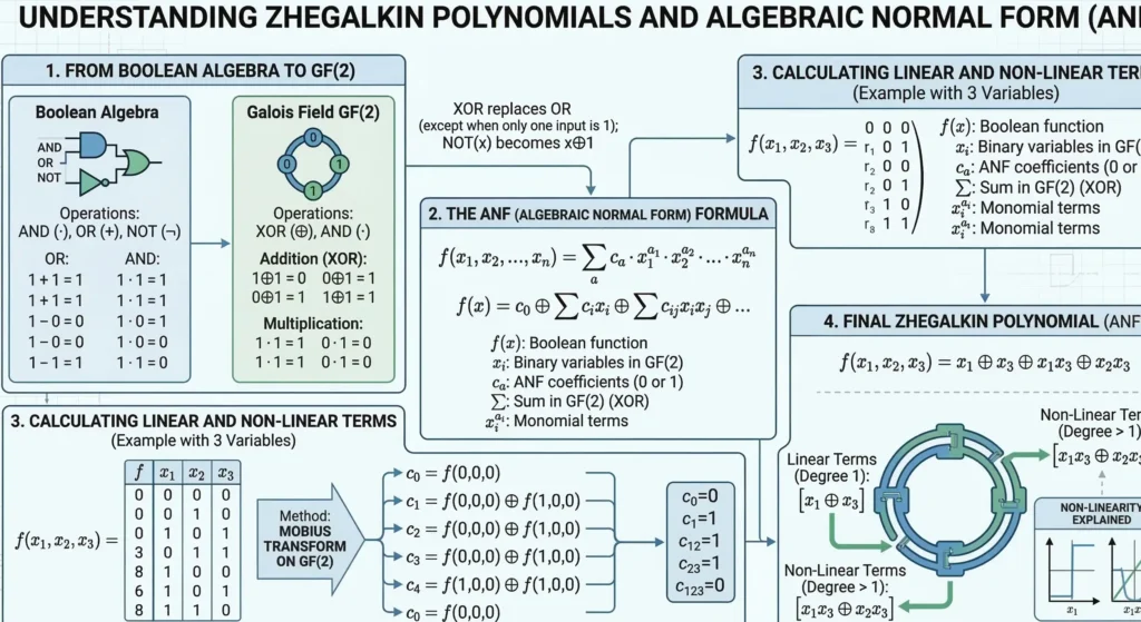
Named after the brilliant mathematician Ivan Zhegalkin, who formalized the concept in 1927, the Zhegalkin polynomial (also known in Western literature as the Algebraic Normal Form, or ANF) is a way to express any logical function using only two operations: Exclusive OR (XOR) and Logical AND (Conjunction).

In this comprehensive guide, we will dive deep into the mathematical mechanics of the Zhegalkin polynomial, explore the critical concept of Boolean linearity within Post’s classes, and teach you two definitive methods for converting any logical formula into its Algebraic Normal Form.

1. The Core Operations: Why Only XOR and AND?

Standard Boolean algebra relies on three primary operators: AND ($\land$), OR ($\lor$), and NOT ($\neg$). However, this system contains redundancies. For example, you can express an OR operation using only AND and NOT via De Morgan’s laws.

Zhegalkin sought to create a system that behaved exactly like traditional polynomial algebra (the math you learned in high school). To do this, he selected operations that perfectly mimic standard addition and multiplication over a field of two elements (the Galois Field $GF(2)$).

Understanding GF(2) in Hardware:

Working within the Galois Field $GF(2)$ isn’t just a mathematical abstraction; it perfectly mirrors how physical silicon chips operate. In this field, there are only two numbers: 0 and 1.

Understanding GF(2) in Hardware:

Working within the Galois Field $GF(2)$ isn’t just a mathematical abstraction; it perfectly mirrors how physical silicon chips operate. In this field, there are only two numbers: 0 and 1.

• Multiplication (AND): Represents two physical switches wired in series. Electricity only flows if switch A and switch B are closed.
• Addition (XOR): Represents a parity checker. XOR evaluates to 1 only if there is an odd number of true inputs. Because of this strict modulo 2 arithmetic, there is no concept of “carrying over” a 1 (like in standard binary addition). This allows cryptographic hardware to execute XOR operations almost instantaneously across 256-bit data blocks without waiting for carry calculations.

• Multiplication is represented by Logical AND ($\land$ or simply $xy$): Just like regular math, $1 \cdot 1 = 1$, and $1 \cdot 0 = 0$.
• Addition is represented by Exclusive OR ($\oplus$):This is also known as addition modulo 2. Unlike the standard logical OR ($\lor$), where $1 \lor 1 = 1$, XOR wraps around like a clock. If you add $1 \oplus 1$, the result is $0$.

Because of this structure, the Zhegalkin polynomial does not use the NOT operator ($\neg$) or the standard OR operator ($\lor$). Everything must be broken down strictly into XOR addition and AND multiplication.

The Magic Property of XOR: Self-Inverse

Before we build a polynomial, you must deeply understand the most important mathematical property of XOR: any variable XORed with itself results in zero.

$$x \oplus x = 0$$

This “self-inverse” property is the secret engine of the Zhegalkin polynomial. It means that during algebraic calculations, identical terms cancel each other out, rapidly shrinking massive equations into elegant, minimized formulas.

2. Anatomy of a Zhegalkin Polynomial

So, what does a Zhegalkin polynomial actually look like? Mathematically, it is a sum (using XOR) of distinct products (using AND). For a function of three variables ($x, y, z$), the most expanded possible polynomial looks like this:

$$f(x, y, z) = a_0 \oplus a_1x \oplus a_2y \oplus a_3z \oplus a_{12}xy \oplus a_{13}xz \oplus a_{23}yz \oplus a_{123}xyz$$

Let’s break down this anatomy:

1. The Constant Term ($a_0$): This can only be a $0$ or a $1$.
2. The Linear Terms: Single variables standing alone ($x$, $y$, $z$).
3. The Non-Linear Terms: Variables multiplied together (conjunctions like $xy$, $xz$, or $xyz$).

The coefficients ($a_i$) are strictly binary ($0$ or $1$). If a coefficient is $1$, that specific term exists in the final polynomial. If it is $0$, the term disappears.

3. Post’s Classes and the Concept of Linearity

Why do computer scientists and cryptographers care so much about calculating the Zhegalkin polynomial? The primary reason is to determine if a Boolean function is linear.

In Emil Post’s functional completeness theory (known as Post’s Lattice), there are five fundamental classes of Boolean functions. One of the most critical is Class L (Linear Functions).

A Boolean function belongs to Class L if and only if its Zhegalkin polynomial contains no multiplied variables.

• Linear Example: $f(x, y, z) = 1 \oplus x \oplus z$ (Notice there are no terms like $xy$. This belongs to Class L).
• Non-Linear Example: $f(x, y, z) = x \oplus yz$ (The presence of $yz$ instantly destroys the linearity. This does not belong to Class L).

[Image comparing a linear Boolean function to a highly non-linear Boolean function using a 3D hypercube]

Why Linearity Matters in the Real World

If you are designing an encryption algorithm to protect banking data, using linear functions is a catastrophic mistake. If an algorithm is strictly linear, an attacker can use linear algebra (like Gaussian elimination) to instantly solve for the secret key. Cryptographers use the Zhegalkin polynomial to mathematically prove that their substitution boxes (S-boxes) contain highly non-linear terms (like $xyz$), making them resistant to advanced mathematical attacks.

4. Method 1: The Algebraic Transformation

If you are given a standard logical formula, you can convert it into a Zhegalkin polynomial using algebraic substitution rules. You must replace every standard operator ($\lor$, $\to$, $\neg$) with its XOR equivalent.

Here is the master cheat sheet for transformations:

• Negation: $\neg x = x \oplus 1$
• Disjunction (OR): $x \lor y = x \oplus y \oplus xy$
• Implication: $x \to y = \neg x \lor y = 1 \oplus x \oplus xy$
• Equivalence: $x \leftrightarrow y = x \oplus y \oplus 1$

Deep Dive: Why does OR become $x \oplus y \oplus xy$? > When converting a standard Disjunction (OR) to Algebraic Normal Form, students often forget the $xy$ term. Why is it there? Think of it through the lens of set theory and the Inclusion-Exclusion principle. An XOR operation ($x \oplus y$) covers the instances where strictly $x$ is true or strictly $y$ is true. However, a standard logical OR also includes the instance where both are true. To correct this missing overlap in our rigid Galois math, we must add the intersection back into the equation (represented by $xy$). Thus, $x \lor y$ perfectly translates to $x \oplus y \oplus xy$

Step-by-Step Algebraic Example

Let’s take a standard Disjunctive Normal Form (DNF) function: $f(x, y) = \neg x \lor (x \land y)$. Let’s convert it.

Step 1: Replace the Negation.

$$f(x, y) = (x \oplus 1) \lor (xy)$$

Step 2: Replace the OR operator.

Using the rule $A \lor B = A \oplus B \oplus AB$, where $A = (x \oplus 1)$ and $B = (xy)$:

$$f(x, y) = (x \oplus 1) \oplus (xy) \oplus ((x \oplus 1)xy)$$

Step 3: Distribute the multiplication.

$$f(x, y) = x \oplus 1 \oplus xy \oplus (x \cdot xy \oplus 1 \cdot xy)$$

Since $x \cdot x = x$ (a variable ANDed with itself is just itself):

$$f(x, y) = x \oplus 1 \oplus xy \oplus x^2y \oplus xy$$

$$f(x, y) = x \oplus 1 \oplus xy \oplus xy \oplus xy$$

Step 4: Cancel out identical XOR terms.

Remember the magic rule: $xy \oplus xy = 0$. We have three $xy$ terms. Two of them cancel out, leaving just one.

$$f(x, y) = 1 \oplus x \oplus xy$$

We have successfully calculated the Zhegalkin polynomial! Because it contains the term $xy$, we also know this function is non-linear.

5. Method 2: The Method of Undetermined Coefficients (Pascal’s Triangle)

Algebraic transformation is great for small formulas, but if you are starting with a truth table, the Pascal’s Triangle Method (also called the Triangle of Truth) is significantly faster and less prone to human error.

Let’s assume we have a function $f(x, y, z)$ whose truth table output vector (from $000$ to $111$) is: [0, 1, 1, 0, 1, 0, 0, 1].

To find the polynomial coefficients using the triangle method:

1. Write the output vector as the top row.
2. To generate the next row down, XOR adjacent elements in the row above it ($0 \oplus 1 = 1$, $1 \oplus 1 = 0$, etc.).
3. Continue building an inverted triangle until you reach a single bit at the bottom.

The Calculation:

Row 1 (Truth Table): 0 1 1 0 1 0 0 1

Row 2 (XOR pairs) : 1 0 1 1 1 0 1

Row 3 (XOR pairs) : 1 1 0 0 1 1

Row 4 (XOR pairs) : 0 1 0 1 0

Row 5 (XOR pairs) : 1 1 1 1

Row 6 (XOR pairs) : 0 0 0

Row 7 (XOR pairs) : 0 0

Row 8 (XOR pairs) : 0

The Mathematical Beauty of the Triangle: This technique is formally known as the Moebius Inversion over a Boolean Hypercube. What you are actually doing when you XOR adjacent bits row by row is calculating the discrete Boolean derivative of the function. Interestingly, if you draw a massive Pascal’s triangle using this exact XOR method (where every number is the sum modulo 2 of the two numbers above it), the resulting pattern of 1s and 0s creates a perfect Sierpinski fractal. This highlights the deep mathematical symmetry underlying Boolean algebra.

Finding the Coefficients:

The coefficients for the Zhegalkin polynomial are simply the first element of every row, reading from top to bottom.

In our case, the left-most edge of the triangle is: [0, 1, 1, 0, 1, 0, 0, 0].

These numbers correspond directly to the canonical terms in binary order ($1, z, y, yz, x, xz, xy, xyz$):

• $a_0 (1) = 0$
• $a_1 (z) = 1$
• $a_2 (y) = 1$
• $a_3 (yz) = 0$
• $a_4 (x) = 1$
• $a_5 (xz) = 0$
• $a_6 (xy) = 0$
• $a_7 (xyz) = 0$

By dropping the terms with a $0$ coefficient, our final Zhegalkin polynomial is perfectly revealed:

$$f(x, y, z) = z \oplus y \oplus x$$

Since there are no multiplied variables (no conjunctions), this specific function belongs to Post’s Class L. It is perfectly linear!

Method 2: The Method of Undetermined Coefficients (Pascal’s Triangle Method)

While algebraic transformation is effective for small formulas, the Pascal’s Triangle Method (also known as the Truth Triangle Method) is significantly faster and less prone to human error when starting from a truth table. This technique is formally known as Moebius Inversion over a Boolean Hypercube. What you are actually doing when you XOR adjacent bits row by row is calculating the discrete Boolean derivative of the function.

To illustrate this method, let us assume we have a function $f(x, y, z)$ whose truth table output vector is: $[0, 1, 1, 0, 1, 0, 0, 1]$.

We will use a detailed, bulletproof three-stage process to arrive at the correct polynomial.

Stage 1: Preparation and Understanding Variable Order

This is the critical foundational stage. An error here guarantees an incorrect final polynomial.

1. Variable Ordering in the Truth Table: By standard convention, a truth table is constructed with variables listed from most significant bit (MSB) to least significant bit (LSB). For $f(x, y, z)$, the MSB is $x$, and the LSB is $z$.
2. Canonical Truth Vector: The truth vector (column of output results) must be written in the canonical order that corresponds to the ascending binary codes of the input variables (from 000 to 111).

Let us write out the complete truth table for this example to clearly see where the vector $[0, 1, 1, 0, 1, 0, 0, 1]$ originates:

Input x	Input y	Input z	Binary Code	Output f(x,y,z)	ANF Polynomial Term
0	0	0	000	0	$a_0 \cdot 1$ (Constant)
0	0	1	001	1	$a_1 \cdot z$
0	1	0	010	1	$a_2 \cdot y$
0	1	1	011	0	$a_3 \cdot yz$
1	0	0	100	1	$a_4 \cdot x$
1	0	1	101	0	$a_5 \cdot xz$
1	1	0	110	0	$a_6 \cdot xy$
1	1	1	111	1	$a_7 \cdot xyz$

Truth Vector ($V$): $[0, 1, 1, 0, 1, 0, 0, 1]$.

Stage 2: Constructing the “Inverted Triangle” (Truth Triangle)

This stage involves purely mechanical calculations. The goal is to derive the coefficients $a_0, a_1, \dots, a_7$.

Calculation Rule:

• Each subsequent row contains one fewer element than the row above it.
• An element in a new row is calculated by performing an XOR (addition modulo 2) operation on the two adjacent elements directly above it.

As a reminder, the XOR table is: ($0 \oplus 0 = 0$, $0 \oplus 1 = 1$, $1 \oplus 0 = 1$, $1 \oplus 1 = 0$).

We perform the calculation step-by-step:

Row 1 (Truth Vector):

0   1   1   0   1   0   0   1

Row 2:

$(0 \oplus 1) = \mathbf{1}, \quad (1 \oplus 1) = \mathbf{0}, \quad (1 \oplus 0) = \mathbf{1}, \quad (0 \oplus 1) = \mathbf{1}, \quad (1 \oplus 0) = \mathbf{1}, \quad (0 \oplus 0) = \mathbf{0}, \quad (0 \oplus 1) = \mathbf{1}$

Result:   1   0   1   1   1   0   1

Row 3:

$(1 \oplus 0) = \mathbf{1}, \quad (0 \oplus 1) = \mathbf{1}, \quad (1 \oplus 1) = \mathbf{0}, \quad (1 \oplus 1) = \mathbf{0}, \quad (1 \oplus 0) = \mathbf{1}, \quad (0 \oplus 1) = \mathbf{1}$

Result:       1   1   0   0   1   1

Row 4:

$(1 \oplus 1) = \mathbf{0}, \quad (1 \oplus 0) = \mathbf{1}, \quad (0 \oplus 0) = \mathbf{0}, \quad (0 \oplus 1) = \mathbf{1}, \quad (1 \oplus 1) = \mathbf{0}$

Result:           0   1   0   1   0

Row 5:

$(0 \oplus 1) = \mathbf{1}, \quad (1 \oplus 0) = \mathbf{1}, \quad (0 \oplus 1) = \mathbf{1}, \quad (1 \oplus 0) = \mathbf{1}$

Result:               1   1   1   1

Row 6:

$(1 \oplus 1) = \mathbf{0}, \quad (1 \oplus 1) = \mathbf{0}, \quad (1 \oplus 1) = \mathbf{0}$

Result:                   0   0   0

Row 7:

$(0 \oplus 0) = \mathbf{0}, \quad (0 \oplus 0) = \mathbf{0}$

Result:                       0   0

Row 8:

$(0 \oplus 0) = \mathbf{0}$

Result:                           0

---

Here is how the complete triangle looks (with the leftmost edge elements highlighted):

Row	Elements
R1	0   1   1   0   1   0   0   1
R2	1   0   1   1   1   0   1
R3	1   1   0   0   1   1
R4	0   1   0   1   0
R5	1   1   1   1
R6	0   0   0
R7	0   0
R8	0

Stage 3: Assembling the Polynomial and Assigning Coefficients

The polynomial coefficients ($a_i$) are simply the first (leftmost) elements of every row in the triangle.

Writing them out from top to bottom, we get:

Coefficient Vector ($A$) = $[0, 1, 1, 0, 1, 0, 0, 0]$.

This gives us values for $a_0, a_1, a_2, a_3, a_4, a_5, a_6, a_7$, respectively.

Mapping Coefficients to Logical Terms:

Mathematical symmetry applies here. The order of the coefficients $a_i$ corresponds directly to the binary code order of the input variables used in Stage 1, which in turn defines which variables exist in each polynomial term. If a binary position is ‘1’, that variable exists in the conjunction.

Mapping them out:

• $a_0$ corresponds to binary code 000: No variables. This is the constant term.
• $a_1$ corresponds to binary code 001: Variable $z$ (unit in the LSB position).
• $a_2$ corresponds to binary code 010: Variable $y$ (unit in the middle position).
• $a_3$ corresponds to binary code 011: Variables $y$ and $z$ ($y \cdot z$).
• $a_4$ corresponds to binary code 100: Variable $x$ (unit in the MSB position).
• $a_5$ corresponds to binary code 101: Variables $x$ and $z$ ($x \cdot z$).
• $a_6$ corresponds to binary code 110: Variables $x$ and $y$ ($x \cdot y$).
• $a_7$ corresponds to binary code 111: Variables $x, y, z$ ($x \cdot y \cdot z$).

We now combine these coefficients with their logical Algebraic Normal Form (ANF) terms:

$$f(x, y, z) = a_0 \oplus a_1z \oplus a_2y \oplus a_3yz \oplus a_4x \oplus a_5xz \oplus a_6xy \oplus a_7xyz$$

Substituting the values from Coefficient Vector $A = [0, 1, 1, 0, 1, 0, 0, 0]$:

$$f(x, y, z) = (0) \oplus (1)z \oplus (1)y \oplus (0)yz \oplus (1)x \oplus (0)xz \oplus (0)xy \oplus (0)xyz$$

Dropping terms with a ‘0’ coefficient yields the final Zhegalkin polynomial:

$$f(x, y, z) = z \oplus y \oplus x$$

We have successfully calculated the polynomial. Because it contains only single variables and no conjunctions (products like $xy$ or $xyz$), we conclude that this function is linear and belongs to Post’s Class $L$.

---

Method Algorithm Summary

1. Preparation: Verify variable ordering (MSB to LSB). Construct the standard truth table and write the output column as a row vector (Truth Vector).
2. Triangle Generation: Generate subsequent rows by XORing adjacent elements from the row above until only one bit remains.
3. Coefficient Extraction: Extract the leftmost edge of the triangle (the first bit of every row) as the Coefficient Vector.
4. ANF Mapping: Map these coefficients in order to the standard ANF terms: constant, $z, y, yz, x, xz, xy, xyz$.
5. Assembly: Construct the final polynomial using only terms with a coefficient of ‘1’, combined via the XOR operator ($\oplus$).

Conclusion: The Bridge to Advanced Computing

The Zhegalkin polynomial is far more than a mathematical curiosity. By forcing Boolean logic into the rigid structure of Galois Field algebra using XOR and AND, computer scientists gain the ability to mathematically prove the security of cryptographic ciphers and optimize digital circuitry.

Whether you choose to use algebraic expansion to carefully unpack the logic, or employ the visual elegance of the Pascal triangle method, calculating the Algebraic Normal Form is an essential skill in discrete mathematics.

Now that we understand how to determine linearity, it is time to expand our toolkit. In our next module, we will explore the rest of Emil Post’s functional completeness theorem, diving into monotonicity, self-duality, and how to prove that a set of logical gates is computationally universal.