1 Best Guide to Adjacency and Incidence Matrices in Graph Theory
If you want to excel in computer science, software engineering, or advanced discrete mathematics, you must learn how computers process complex networks. While humans can look at a visual diagram of interconnected dots and lines to find a path, a computer processor relies purely on numbers, memory addresses, and data structures. To bridge this gap, engineers primarily rely on adjacency and incidence matrices.
In our previous lesson, Set Theory Operations and Venn Diagrams, we learned how to group abstract elements. Now, Graph Theory takes those sets and strictly defines the dynamic relationships between them. A graph $G = (V, E)$ consists of Vertices ($V$) and Edges ($E$). When these edges have a strict one-way direction (like a one-way street), the structure is called a Directed Graph or Digraph. But how do we store this digraph in RAM? The most mathematical approach is using adjacency and incidence matrices.
In this comprehensive, deep-dive guide, we will strictly define adjacency and incidence matrices, walk through a practical 7-vertex diagram example, and—crucially for technical coding interviews—introduce the highly optimized Adjacency List alternative.
1. The Foundation: Why Matrices Matter in Graph Theory
Whenever you request a route on Google Maps, analyze a social media friend network, or compile source code, a graph algorithm is executing in the background. Graph algorithms (like Dijkstra’s shortest path or Depth-First Search) require rapid access to node connections. By translating visual arrows into 2D arrays (tables of numbers), adjacency and incidence matrices allow $O(1)$ constant-time lookups to determine if two nodes are connected.
Understanding the exact differences between adjacency and incidence matrices is a mandatory requirement for passing algorithmic coding interviews at top tech companies. Let us break down both data structures mathematically.
2. The Adjacency Matrix (Vertex-to-Vertex Mapping)
The first of our adjacency and incidence matrices is the Adjacency Matrix. It is the most intuitive way to represent a graph in computer memory. It answers one fundamental question instantly: “Is there a direct, unbroken path starting from Vertex $i$ and ending at Vertex $j$?”
Mathematical Definition and Matrix Structure
An Adjacency Matrix is always a square matrix of size $|V| \times |V|$, where $|V|$ represents the total number of vertices (nodes) in the graph. The rows represent the origin vertices (where the arrow starts), and the columns represent the destination vertices (where the arrow ends).
For an unweighted directed graph, the elements of the matrix, denoted algebraically as $A_{ij}$, are populated using strict boolean (binary) logic:
- $A_{ij} = 1$: If there is a directed edge pointing from vertex $i$ strictly to vertex $j$.
- $A_{ij} = 0$: If there is absolutely no direct edge pointing from vertex $i$ to vertex $j$.
Key Algorithmic Properties of the Adjacency Matrix
When studying adjacency and incidence matrices, knowing their computational traits is vital:
- Asymmetry in Digraphs: In a directed graph, the matrix is rarely symmetrical. An edge from node 2 to node 1 ($A_{2,1} = 1$) does not imply an edge from 1 to 2 ($A_{1,2}$ might be 0).
- The Main Diagonal: The diagonal entries ($A_{1,1}, A_{2,2}, \dots$) remain 0 unless the specific node has a “self-loop” (an arrow pointing back to itself).
- Out-degree Calculation: Summing the values across an entire row calculates the out-degree of that vertex (total departing arrows).
- In-degree Calculation: Summing the values down an entire column reveals the in-degree (total arriving arrows).
- Space Complexity: The memory required is strictly $O(|V|^2)$. If you have 10,000 users in a database, the matrix requires 100,000,000 memory slots, even if users only have 2 friends each.
3. The Incidence Matrix (Vertex-to-Edge Mapping)
The second pillar in our study of adjacency and incidence matrices is the Incidence Matrix. While the adjacency model focuses strictly on how vertices relate to other vertices, the Incidence Matrix maps vertices directly to specific edges. It answers the question: “What is the exact physical relationship between this specific vertex and this specific edge?”
Mathematical Definition and Matrix Structure
An Incidence Matrix is a rectangular matrix of size $|V| \times |E|$, where $|V|$ is the number of vertices (rows) and $|E|$ is the number of edges (columns). Edges are typically assigned unique identifiers like letters ($a, b, c$).
For a directed graph, the elements of the matrix, denoted as $M_{ij}$, use a trinary system to capture the flow of direction:
- $M_{ij} = 1$: The edge $j$ leaves (originates from) vertex $i$.
- $M_{ij} = -1$: The edge $j$ enters (terminates at) vertex $i$.
- $M_{ij} = 0$: The edge $j$ has no physical connection to vertex $i$.
Key Algorithmic Properties of the Incidence Matrix
When comparing adjacency and incidence matrices, the incidence matrix has unique mathematical quirks:
- The Zero-Sum Rule: In a standard directed graph without self-loops, every edge must originate exactly once ($+1$) and terminate exactly once ($-1$). Therefore, the sum of any column in an Incidence Matrix will always equal exactly zero.
- Space Complexity: The memory required is $O(|V| \times |E|)$.
- Application: To explore deeper applications of incidence matrices in electrical engineering, you can read the Wikipedia documentation on incidence metrics, which explains Kirchhoff’s circuit laws.
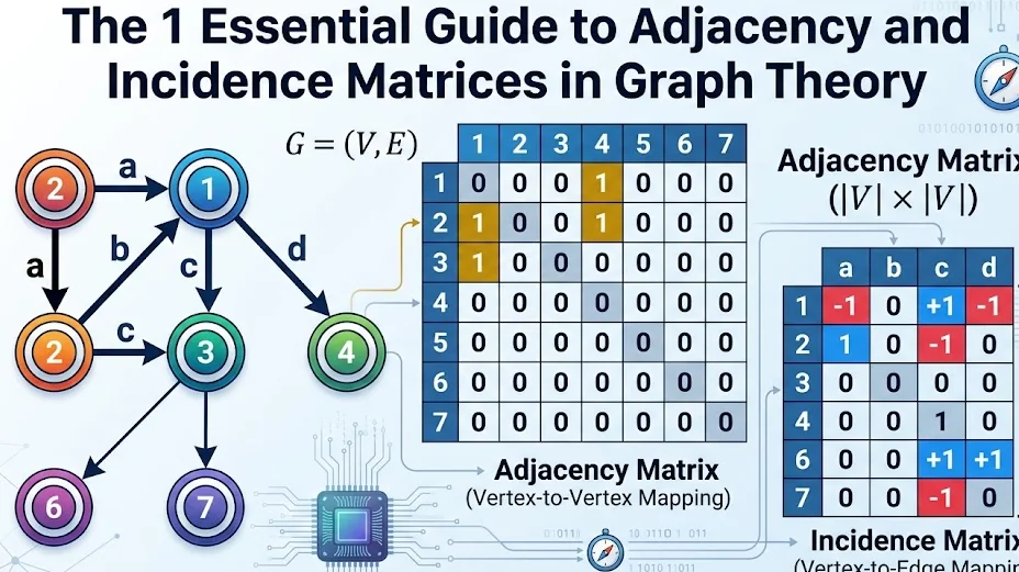
4. Practical Step-by-Step Problem: The 7-Vertex Graph
To truly comprehend adjacency and incidence matrices, we must apply the theory to a tangible discrete mathematics problem. Let us manually compile these matrices for a directed graph featuring 7 vertices and a specific edge labeled $a$.
The Known Graph Data:
- Vertices ($V$): $\{1, 2, 3, 4, 5, 6, 7\}$
- Edge of Interest ($a$): A directed arrow originates at Vertex 2 and points downward to terminate at Vertex 1.
Compiling the Adjacency Matrix Data
We are building a $7 \times 7$ grid. How do we record the presence of edge $a$?
- Identify the Origin: The arrow begins at Vertex 2. We navigate to Row 2.
- Identify the Target: The arrow points to Vertex 1. We navigate to Column 1.
- Apply the Binary Rule: At the precise intersection of Row 2 and Column 1 ($A_{2,1}$), we write the integer 1.
Assuming no other edges leave Vertex 2, the complete sequence for Row 2 would be: [1, 0, 0, 0, 0, 0, 0].
Compiling the Incidence Matrix Data
Now, we build a matrix where rows are vertices 1 through 7, but the columns are the edges. Let us strictly analyze the column dedicated to edge $a$.
- Departure Point: Edge $a$ leaves Vertex 2. Outgoing edges are positive. In Row 2 of Column $a$, we write 1.
- Arrival Point: Edge $a$ enters Vertex 1. Incoming edges are negative. In Row 1 of Column $a$, we write -1.
- Unconnected Vertices: Edge $a$ never touches vertices 3, 4, 5, 6, or 7. Rows 3 through 7 in Column $a$ all receive a 0.
Reading the column for edge $a$ from top to bottom yields: [-1, 1, 0, 0, 0, 0, 0]. This column perfectly isolates the physical lifecycle of that single connection.
5. The Adjacency List: The Coding Interview Champion
While theoretical mathematics focuses heavily on adjacency and incidence matrices, modern software engineering often avoids them in favor of a third structure: the Adjacency List. If you are preparing for a technical coding interview at FAANG, understanding why Adjacency Lists usually beat adjacency and incidence matrices is essential.
The Problem with Matrices in Programming
In the real world, most networks are “Sparse Graphs.” Think of Facebook: out of 3 billion users, the average person has maybe 300 friends. If you use an Adjacency Matrix, you have to allocate $3 \text{ billion} \times 3 \text{ billion}$ slots in memory, and 99.9999% of those slots will just hold the number 0. This is a catastrophic waste of RAM.
How the Adjacency List Works
Instead of building a massive 2D grid of adjacency and incidence matrices, an Adjacency List uses an Array (or Hash Map) where each index represents a vertex. The value stored at that index is simply a Linked List (or dynamic array) containing only the vertices it is actually connected to.
For our 7-vertex graph, where Vertex 2 points to Vertex 1, the Adjacency List looks like this in code:
Graph_List = {
    1: [],          // Vertex 1 points to nothing
    2: [1],         // Vertex 2 points to Vertex 1
    3: [],
    4: [],
    ...
}
Why Adjacency Lists Win in Technical Interviews
- Optimal Space Complexity: Instead of $O(|V|^2)$ memory, an Adjacency List requires only $O(|V| + |E|)$ space. You only pay for the edges that actually exist.
- Faster Traversal: Algorithms like Breadth-First Search (BFS) and Depth-First Search (DFS) run significantly faster using lists because they do not have to iterate over thousands of
0s just to find the next valid edge. You can learn more about standard graph traversals via GeeksforGeeks graph algorithms tutorials.
6. Comparing Matrices vs. Lists: Which to Choose?
To master graph data structures, you must know when to utilize adjacency and incidence matrices versus lists. Below is a professional breakdown of their computational trade-offs:
| Data Structure | Space Complexity | Check if Edge Exists | Iterate Over Neighbors | Best Use Case |
|---|---|---|---|---|
| Adjacency Matrix | $O(|V|^2)$ | $O(1)$ (Instant) | $O(|V|)$ (Slow) | Dense graphs, minimal vertices, quick lookups. |
| Incidence Matrix | $O(|V| \times |E|)$ | $O(|E|)$ | $O(|E|)$ | Electrical network topologies, circuit states. |
| Adjacency List | $O(|V| + |E|)$ | $O(\text{degree})$ | $O(\text{degree})$ (Fast) | Sparse graphs, social networks, algorithms (DFS/BFS). |
Conclusion: The Future of Network Routing
From routing internet packets across global servers to mapping chemical bonds in molecular biology, graph theory drives the modern world. Translating visual dots and arrows into rigorous adjacency and incidence matrices is the necessary first step to making these networks comprehensible to computer hardware.
While mathematical textbooks will heavily focus on adjacency and incidence matrices to prove theorems, your future career as a developer will require you to seamlessly switch between matrices and Adjacency Lists depending on the strict memory constraints of the system you are building. Check out our Advanced Data Structures Guide to continue mastering memory optimization techniques!