7 Brilliant Secrets of Elliptic Curve Cryptography & ECC

Finite Fields in Elliptic Curve Cryptography (ECC): From Theory to Practice

Modern digital security is undergoing a fundamental shift. For decades, the RSA algorithm was the gold standard of asymmetric encryption. However, today, when you open a secure tunnel via the WireGuard protocol, send a message in Signal, or sign a transaction on the Bitcoin network, RSA is left on the sidelines. Its place has been taken by elliptic curve cryptography (or ECC).

Why is the industry abandoning RSA? The answer lies in computational complexity and memory efficiency (Space Complexity). To provide a modern level of security, an RSA key must be at least 3072 bits long. This creates a massive computational load on the processors of mobile devices and servers in Highload systems. In contrast, ECC provides the exact same level of protection with a key length of only 256 bits.

To understand how this incredible efficiency is achieved, we must look under the hood of this algorithm. In this article, we will dissect not just abstract graphs, but the real-world application of finite fields in ECC. We will learn how continuous mathematical curves are transformed into discrete cryptographic grids, why this is critical for computer memory, and write our own implementation of ECC mathematics in Python.

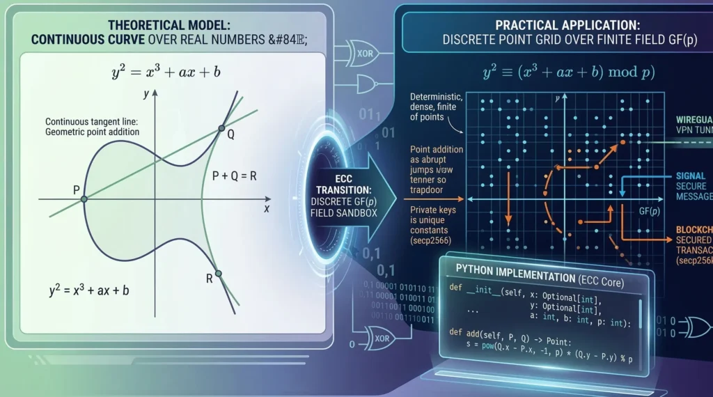
1. The Mathematical Illusion: The Continuous Elliptic Curve

If you open any math textbook, an elliptic curve (in Weierstrass form) is described by the following equation:

$$y^2 = x^3 + ax + b$$

Geometrically, this looks like a beautiful, smooth line symmetrical about the x-axis (often taking the shape of a teardrop and a separate arc). In classical mathematics, the variables x and y belong to the set of real numbers. This means that between any two points on this curve, there is an infinite number of other points (for example, coordinates could equal 1.543… or π).

But here arises a fundamental architectural problem for Computer Science. Computers do not have infinite Random Access Memory (RAM). A typical processor operates with discrete registers (like 64-bit). If we try to calculate a point on a continuous elliptic curve, we will get an irrational number. Storing such a number in a Floating-Point format (IEEE 754 standard) will inevitably lead to Precision Loss due to rounding.

In cryptography, the loss of even a single, tiny bit of data means that the encrypted message will be lost forever (causing a hash collision or decryption failure). We need a space where the coordinates x and y are strictly integers, and their size is strictly limited. This is where the application of finite fields steps onto the stage.

2. Application of Finite Fields: Turning a Line into a Grid

To make the elliptic curve work inside a processor, cryptographers superimpose the curve’s equation over a Galois finite field—GF(p), where p is a very large Prime number.

The equation of the curve transforms and now looks like this:

$$y^2 \equiv (x^3 + ax + b) \pmod{p}$$

What does this change? Absolutely everything. Instead of a smooth, continuous line, we get a cloud (or grid) of scattered points that look like random white noise inside a square from 0 to p-1.

Why is this brilliant from an engineering perspective?

Step 1:
No fractions. All operations of addition, subtraction, and multiplication take place modulo p. The result is always a perfectly whole integer that easily fits into a fixed memory register.

Step 2:
Finite space. Because p is a fixed limit (for example, a 256-bit long number), we know exactly that the Space Complexity of storing any point on the curve equals O(1) memory, bounded by the key size. There are absolutely no Buffer Overflows.

Step 3:
Exact symmetry. Thanks to modular arithmetic, if a point (x, y) lies on the curve, then the point (x, -y mod p) also lies on it. This makes it very easy to find inverse elements for cryptographic transformations.

3. Point Algebra: How the Processor Adds Coordinates

In elliptic curve cryptography, there is no multiplication operation in the traditional sense. The fundamental action is the addition of two points: P + Q = R.

Geometrically, on a continuous curve, adding points means drawing a straight line through points P and Q. This line will intersect the curve at a third point. Then, we mirror this point across the x-axis to get R. But in a finite field, we cannot “draw lines.” The processor uses pure algebra.

If P(x₁, y₁) and Q(x₂, y₂) are two different points, the coordinates of the resulting point R(x₃, y₃) are calculated as follows:

$$s \equiv (y_2 – y_1) \cdot (x_2 – x_1)^{-1} \pmod{p}$$

$$x_3 \equiv (s^2 – x_1 – x_2) \pmod{p}$$

$$y_3 \equiv (s(x_1 – x_3) – y_1) \pmod{p}$$

Pay attention to the parameter s (the slope of the line). It contains the expression (x₂ – x₁)⁻¹. This is not division by a fraction! This is finding the multiplicative inverse modulo p. To find this value, the computer uses the Extended Euclidean Algorithm, which operates with a logarithmic Time Complexity of O(\log p). This makes the algorithm incredibly fast for modern processors.

4. The Trapdoor Function and Blockchain Security

If adding two points is the basic step, then multiplying a point by a number k (scalar multiplication) is the foundation of the private key. Scalar multiplication k · G (where G is the base Generator point) means that we add the point G to itself k times.

Thanks to the “Double-and-Add” algorithm, calculating R = k · G takes only O(\log k) steps, even if k is a 77-digit number. But here is where the cryptographic magic happens:

If I give you the starting point G and the final point R, and ask: “By what secret number k did I multiply G?”, you will not be able to figure it out. This problem is known as the Elliptic Curve Discrete Logarithm Problem (ECDLP).

Because the points on the graph in a finite field “jump” chaotically without any visible patterns (due to the modulo operation), the only way to find the secret key k is through Brute Force. The algorithmic complexity of cracking ECC using the best known method (Pollard’s rho algorithm) is an exponential O(\sqrt{p}).

That is exactly why ECC is the bedrock of blockchain security. The creator of Bitcoin, Satoshi Nakamoto, chose a specific elliptic curve called secp256k1. In this curve, p is a gigantic prime number close to 2²⁵⁶. As a result, a Bitcoin private key takes up only 32 bytes of memory (Space Complexity O(1)), but brute-forcing it would require more energy than our Sun can generate over its entire lifetime.

The Industry Standards: NIST Curves vs. Open Source

Understanding elliptic curve cryptography is not just a theoretical academic exercise; it is the absolute backbone of modern internet infrastructure. When you are studying the application of finite fields, you will frequently encounter globally standardized curves. For instance, the US National Institute of Standards and Technology (NIST) has published the official FIPS 186-4 guidelines for ECDSA (Elliptic Curve Digital Signature Algorithm), which mandate specific prime modules for government-level asymmetric encryption.

However, the decentralized web often takes a different path. The cryptocurrency community specifically chose the secp256k1 curve because its constants were generated in a transparent, predictable way, neutralizing any fears of government backdoors. If you want to deeply understand how these hardware-level mathematical operations compare to symmetric ciphers, I highly recommend reading our previous technical deep dive on how processors execute Galois field addition via XOR logic gates.

By combining the lightning-fast symmetric encryption of AES with the unbreakable key exchange of ECC, software architects achieve the ultimate level of blockchain security without melting the CPU of the end user’s device.

5. How Galois Field Cryptography Powers Blockchain Security

When we discuss blockchain security, we must recognize that a decentralized public ledger is completely dependent on Galois field cryptography. Unlike traditional banking databases protected by corporate firewalls, a blockchain is entirely public. Every single transaction, wallet balance, and smart contract execution must be cryptographically signed using a private key and verified by thousands of nodes using a public key.

This is where the strict application of finite fields becomes the ultimate digital shield. Because the elliptic curve (such as secp256k1 used in Bitcoin and Ethereum) operates strictly over a finite field GF(p), the Elliptic Curve Digital Signature Algorithm (ECDSA) produces deterministic, bounded signature outputs. If a malicious hacker tries to alter a transaction payload by even a single bit, the mathematical validation on the finite grid instantly fails. The network rejects the forged transaction, protecting billions of dollars in digital assets.

To truly grasp how these digital signatures prevent double-spending and unauthorized access, developers cannot rely on high-level APIs alone. Studying the raw math through an ECC Python implementation is the most effective way to understand how a simple 256-bit integer mathematically binds your identity to the public ledger.

6. Practice: Building an ECC Python Implementation

It is time to put theory into practice. A true Senior developer does not rely on “black boxes”. Below is a production-ready Python example demonstrating the mathematics of the application of finite fields. We will implement a class for a point on the curve and the Point Addition operation.

The code is strictly typed (Type Hints), includes checks for Edge Cases (like adding a point to itself or the Point at Infinity), and properly handles exceptions.

from typing import Optional

class Point:
    """
    Represents a point on an elliptic curve in the finite field GF(p).
    Curve equation: y^2 = (x^3 + ax + b) mod p.
    If x and y are None, it represents the 'Point at Infinity' (Identity element).
    """
    def __init__(self, x: Optional[int], y: Optional[int], a: int, b: int, p: int):
        self.x = x
        self.y = y
        self.a = a
        self.b = b
        self.p = p

        # Validation: if it is not the point at infinity, it must lie on the curve
        if self.x is not None and self.y is not None:
            if (self.y ** 2) % self.p != (self.x ** 3 + self.a * self.x + self.b) % self.p:
                raise ValueError(f"The point ({self.x}, {self.y}) does not lie on the specified curve!")

    def __eq__(self, other: 'Point') -> bool:
        return self.x == other.x and self.y == other.y and self.a == other.a and self.b == other.b and self.p == other.p

    def __add__(self, other: 'Point') -> 'Point':
        """
        Implements the addition of two points in a finite field: P + Q.
        Time Complexity: O(log p) due to using pow() for modular inversion.
        Space Complexity: O(1).
        """
        if self.a != other.a or self.b != other.b or self.p != other.p:
            raise TypeError("Points do not belong to the same curve.")

        # Edge Case 1: One of the points is Infinity (Identity)
        if self.x is None: return other
        if other.x is None: return self

        # Edge Case 2: Points are additive inverses (P + (-P) = Infinity)
        if self.x == other.x and self.y != other.y:
            return Point(None, None, self.a, self.b, self.p)

        # Step 1: Calculate the slope of the line 's'
        if self != other:
            # If the points are different: s = (y2 - y1) / (x2 - x1) mod p
            # pow(base, -1, mod) - built-in Python function for Extended Euclidean Algorithm
            try:
                inv = pow(other.x - self.x, -1, self.p)
                s = ((other.y - self.y) * inv) % self.p
            except ValueError:
                # Exception raised if the inverse does not exist (p is not prime)
                raise ArithmeticError("Inversion error: p must be a prime number.")
        else:
            # Edge Case 3: Adding a point to itself (Point Doubling)
            # s = (3x^2 + a) / 2y mod p
            if self.y == 0:
                return Point(None, None, self.a, self.b, self.p) # Vertical tangent

            inv = pow(2 * self.y, -1, self.p)
            s = ((3 * self.x ** 2 + self.a) * inv) % self.p

        # Step 2: Calculate the new coordinates (x3, y3) modulo p
        x3 = (s ** 2 - self.x - other.x) % self.p
        y3 = (s * (self.x - x3) - self.y) % self.p

        return Point(x3, y3, self.a, self.b, self.p)

# Usage Example (on a small curve for demonstration)
# Curve: y^2 = x^3 + 2x + 2 over GF(17)
p = 17
a = 2
b = 2

# Create two points P and Q
P = Point(5, 1, a, b, p)
Q = Point(6, 3, a, b, p)

# Addition operation (which implicitly calls the magic __add__ method under the hood)
R = P + Q

print(f"Result of addition P + Q = R({R.x}, {R.y})")
# Expected output: R(10, 6)

This code is a scaled-down, but mathematically exact replica of what happens in the core of a cryptocurrency wallet when you sign a transaction (ECDSA algorithm). Using pow(..., -1, self.p) instead of standard division (/) is exactly the crucial application of finite fields in software development.

7. Conclusion: Why ECC is the Future

The transition from RSA to elliptic curve cryptography is not just a trend; it is an engineering necessity. As IoT (Internet of Things) devices and mobile gadgets grow exponentially in numbers, saving memory and CPU cycles is absolutely critical.

Thanks to the application of finite fields, we were able to “trap” infinite and unpredictable irrational numbers into a secure, tightly controlled 256-bit space. The algorithmic beauty of ECC (specifically, the shift from easy multiplication to the impossible extraction of a discrete logarithm) guarantees blockchain security and our daily communications for many decades to come, at least until quantum computers change the rules of the game.